Contents
In this article I have a play with PyEphem and our local star, both as an opportunity to draw some pretty graphs and answer a few basic astronomy related questions, such as: what does the equation of time look like and is there a difference in the time it takes for the sun to set during the year.
Setting up the observer
Import the libraries I am going to need and then set up the observer; I require a latitude, longitude and date as a minimum.
# Import some bits
import ephem, math, datetime
# Get retina display quality for plots
%config InlineBackend.figure_format = 'retina'

home = ephem.Observer()
# Set up
home.date = '2017-01-01 09:00:00'
home.lat = '53.4975'
home.lon = '-0.3154'
Note that the standard and unmodified object has an elevation of 0.0m, temperature of 15.0 degrees Celsius and a pressure of 1010.0 millibars. I did wonder whether or not changing these values would make any difference to the various calculations. Maybe later...
home.elev
0.0
home.temp
15.0
home.pressure
1010.0
Let’s set up the sun next and then compute it from the observer’s position.
Fun with the Sun
Setting up the sun is easy, just:
sun = ephem.Sun()
sun.compute(home)
Rising, Transit & Setting
From there we can get information regarding (from the observer’s point of view) when the last sunrise was, when local noon will occur and when the next sunset is:
rising = home.previous_rising(sun).datetime()
print('Sunrise is at {}:{}:{}'.format(rising.hour, rising.minute, rising.second))

transit = home.next_transit(sun).datetime()
print('Local noon is at {}:{}:{}'.format(transit.hour, transit.minute, transit.second))

setting = home.next_setting(sun).datetime()
print('Sunset is at {}:{}:{}'.format(setting.hour, setting.minute, setting.second))
Sunrise is at 8:16:47
Local noon is at 12:4:56
Sunset is at 15:53:17
Apparent Solar Time
As our Earth does not have a perfectly circular orbit around the sun, the sun is not exactly due south (otherwise known as a transit) every day at 12:00. Depending on the time of year it can be as much as 16 minutes early or late, equating to almost 4° west or east from due south. Let’s draw a graph to illustrate what’s known as the equation of time.
import matplotlib.pyplot as plt
import pandas as pd
import matplotlib
matplotlib.style.use('ggplot')

# Prepare
home.date = '2017/1/1'
sun = ephem.Sun()
times = []

def get_diff(tm):
    """Return a difference in seconds between tm and 12:00:00 on tm's date"""
    a = datetime.datetime.combine(tm, datetime.time(12, 0))
    return (a-tm).total_seconds()/60

# Prepare the data
for i in range(1, 368):
    home.date += ephem.Date(1)
    trans = home.next_transit(sun).datetime()
    times.append(get_diff(trans))

# Set up
ts = pd.Series(times, index=pd.date_range('2017/1/1', periods=len(times)))
What are we doing above? Well we are graphing the difference between the time of the transit of the Sun at the home location and the local time. Let’s have a look at a slice of ts:
ts.loc['2017-04-14':'2017-04-26']
2017-04-14   -1.234778
2017-04-15   -0.997353
2017-04-16   -0.766400
2017-04-17   -0.542189
2017-04-18   -0.324979
2017-04-19   -0.115009
2017-04-20    0.087500
2017-04-21    0.282349
2017-04-22    0.469363
2017-04-23    0.648394
2017-04-24    0.819315
2017-04-25    0.982023
2017-04-26    1.136433
Freq: D, dtype: float64
Go ahead and run the plot:
ax = ts.plot()
plt.rcParams["figure.figsize"] = [9, 6]
ax.set_xlabel(u'Date', fontsize=11)
ax.set_ylabel(u'Variation (minutes)', fontsize=11)
# Fire
plt.show()

So you can see that there are only 4 points in the year where local noon and the sun actually intersect!
Drawing the Analemma
An analemma is the shape the sun will trace out if you were to note its position in the sky at the same time of day once a week over the passage of a year. The shape is a combination of the equation of time and the Earth’s passage around the sun.
Local Noon
Let’s have a go at drawing the analemma occurring at home at local noon (12:00:00):
# Prepare
home.date = '2017/1/1 12:00:00'
sun = ephem.Sun()
posx = []
posy = []

# Solstice altitude
phi = 90 - math.degrees(home.lat)
# Earth axial tilt
epsilon = 23.439

def get_sun_az(tm):
    """Get the azimuth based on a date"""
    sun.compute(tm)
    return math.degrees(sun.az)

def get_sun_alt(tm):
    """Get the altitude based on a date"""
    sun.compute(tm)
    return math.degrees(sun.alt)

# Prepare the data
for i in range(1, 368):
    home.date += ephem.Date(1)
    trans = home.next_transit(sun).datetime()
    posx.append(get_sun_az(home))
    posy.append(get_sun_alt(home))

# Set up
fig, ax = plt.subplots()
ax.plot(posx, posy)
ax.grid(True)
ax.set_xlabel(u'Azimuth (°)', fontsize=11)
ax.set_ylabel(u'Altitude (°)', fontsize=11)
# Add some labels, lines & resize
ax.annotate('Vernal equinox', xy=(min(posx), phi + 1), xytext=(min(posx), phi + 1))
ax.annotate('Autumnal equinox', xy=(max(posx) -2, phi + 1), xytext=(max(posx) -2, phi + 1))
ax.annotate('Nothern solstice', xy=(180.1, phi + epsilon + 1), xytext=(180.1, phi + epsilon + 1))
ax.annotate('Southern solstice', xy=(180.1, phi - epsilon - 2), xytext=(180.1, phi - epsilon - 2))
plt.plot((min(posx), max(posx)), (phi + epsilon, phi + epsilon), 'blue')
plt.plot((min(posx), max(posx)), (phi, phi), 'pink')
plt.plot((min(posx), max(posx)), (phi - epsilon, phi - epsilon), 'green')
plt.axvline(180, color='yellow')
plt.rcParams["figure.figsize"] = [9, 6]
plot_margin = 4
x0, x1, y0, y1 = plt.axis()
plt.axis((x0, x1, y0 - plot_margin, y1 + plot_margin))
# Fire
plt.show()

Changing the time of day we view the analemma
If we change the time of day the analemma is generated at (say 08:30:00) a very different picture emerges:
# Prepare
home.date = '2017/1/1 08:30:00'
home.horizon = '0'
sun = ephem.Sun()
posy = []
posx = []

def get_sun_az(tm):
    """Get the azimuth based on a date"""
    sun.compute(tm)
    return math.degrees(sun.az)

def get_sun_alt(tm):
    """Get the altitude based on a date"""
    sun.compute(tm)
    return math.degrees(sun.alt)

# Prepare the data
for i in range(1, 368):
    home.date += ephem.Date(1)
    posy.append(get_sun_alt(home))
    posx.append(get_sun_az(home))

# Set up
fig, ax = plt.subplots()
ax.plot(posx, posy)
# Add some labels & resize
ax.set_xlabel(u'Azimuth (°)', fontsize=11)
ax.set_ylabel(u'Altitude (°)', fontsize=11)
plt.rcParams["figure.figsize"] = [9, 6]
# Fire
plt.show()
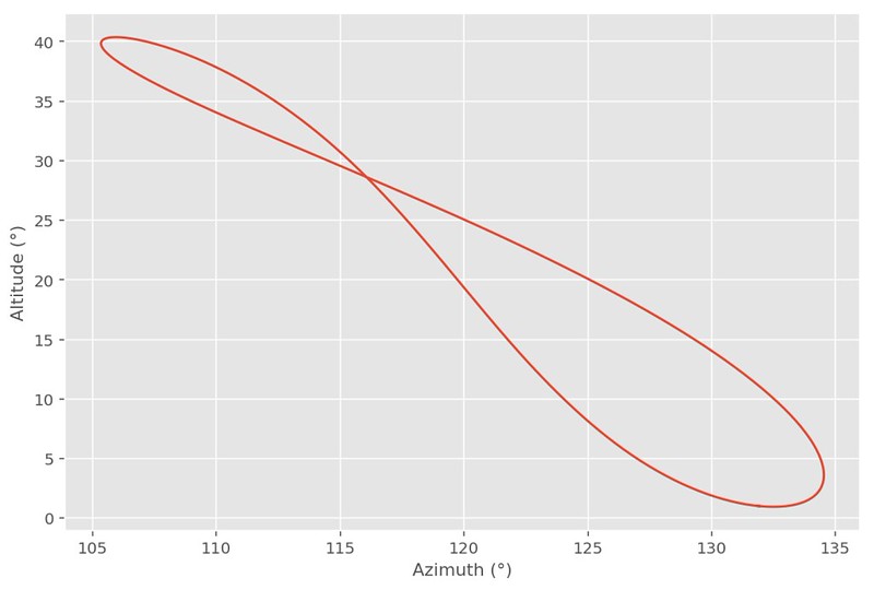
As can be seen above, at mid December southern solstice the Sun is only just above the horizon (bottom right on the graph) and almost due south-east (135°) in direction. By contrast at northern solstice in June the Sun is more or less at 40° and not all that far off due east in direction (top left on the graph).
Calculating Twilights
Which twilight, you might ask. Quite rightly so as there are many definitions:
- Civil twilight
- Nautical twilight
- Astronomical twilight
Civil twilight is defined by the centre of the sun being 6° below the horizon. Under clear conditions bright planets like Venus are easily seen in the sky.
Nautical twilight is defined by the centre of the sun being 12° below the horizon. If the sun is lower it becomes impossible to navigate at sea using the horizon.
Astronomical twilight is defined by the centre of the sun being 18° below the horizon. At this point it becomes quite easy to see stars and other objects under clear sky conditions.
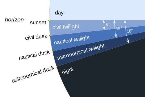
Twilight illustration
By TWCarlson (Own work) [CC BY-SA 3.0 ( http://creativecommons.org/licenses/by-sa/3.0) or GFDL ( http://www.gnu.org/copyleft/fdl.html)], via Wikimedia Commons
Aside: Where on the Disc?
Let’s have a look a twilight calculations using ephem. By default, ephem uses the edge of the sun’s disc for sunset / sunrise calculations; standard definitions use the centre of the sun’s disc. What is the difference between using the edge of the sun and the centre of the sun’s disc to calculate when ordinary (zero degrees horizon) twilight occurs?
initial_set = home.next_setting(sun).datetime() # zero edge
next_set = home.next_setting(sun, use_center=True).datetime() # zero centre

print('Centre sunset is at {}:{}:{}'.format(next_set.hour, next_set.minute, next_set.second))
print('Edge sunset is at {}:{}:{}'.format(initial_set.hour, initial_set.minute, initial_set.second))

delta = initial_set - next_set
print('Time difference is {} mins, {} secs'.format(delta.seconds/60, delta.seconds%60))
Centre sunset is at 15:52:26
Edge sunset is at 15:55:20
Time difference is 2.9 mins, 54 secs
The Calculations
Okay, so let’s write up a basic method to print the different twilight times and how long after normal twilight they occur. The method below yields the amount of time in seconds it takes the Sun to move from sunset on the horizon to positions below the horizon of -6°, -12° and -18° respectively:
def get_setting_twilights(obs, body):
    """Returns a list of twilight datetimes in epoch format"""
    results = []
    # Twilights, their horizons and whether to use the centre of the Sun or not
    twilights = [('0', False), ('-6', True), ('-12', True), ('-18', True)]
    for twi in twilights:
        # Zero the horizon
        obs.horizon = twi[0]
        try:
            # Get the setting time and date
            now = obs.next_setting(body, use_center=twi[1]).datetime()
            # Get seconds elapsed since midnight
            results.append(
                (now - now.replace(hour=0, minute=0, second=0, microsecond=0)).total_seconds()
            )
        except ephem.AlwaysUpError:
            # There will be occasions where the sun stays up, make that max seconds
            results.append(86400.0)
    return results

home.horizon = '0'
twilights = get_setting_twilights(home, sun)
twilights
[57320.284733, 59906.438312, 62546.839518, 65098.990754]
Now we can get started on calculating some twilights at the home location. First reset the date to the first day of 2017, set the horizon to zero degrees, set up a sun body and then off we go:
# Prepare
home.date = '2017/01/01 12:00:00'
home.horizon = '0'
sun = ephem.Sun()
twidataset = []

# Calculate just over a year of data
for i in range(1, 368):
    home.date += ephem.Date(1)
    twidataset.append(get_setting_twilights(home, sun))
What does twidataset contain? Well, it is just a list of lists for now as can be seen from the slice below:
twidataset[150:160]
[[73229.081533, 76304.927372, 81102.660945, 86400.0],
 [73298.278985, 76390.550644, 81255.72959, 86400.0],
 [73365.046584, 76473.20831, 81405.712504, 86400.0],
 [73429.309671, 76552.779425, 81552.226662, 86400.0],
 [73490.995712, 76629.145042, 81694.856699, 86400.0],
 [73550.034189, 76702.188545, 81833.158322, 86400.0],
 [73606.356557, 76771.796561, 81966.651319, 86400.0],
 [73659.896242, 76837.858304, 82094.829296, 86400.0],
 [73710.588832, 76900.266566, 82217.151337, 86400.0],
 [73758.372248, 76958.918635, 82333.05185, 86400.0]]
I’m now going to change the list into a pandas DataFrame object:
df = pd.DataFrame(twidataset, columns=['Sunset', 'Civil', 'Nautical', 'Astronomical'])
Let’s have a peek at a slice of the data frame:
df[150:160]
| Sunset | Civil | Nautical | Astronomical | |
|---|---|---|---|---|
| 150 | 73229.081533 | 76304.927372 | 81102.660945 | 86400.0 |
| 151 | 73298.278985 | 76390.550644 | 81255.729590 | 86400.0 |
| 152 | 73365.046584 | 76473.208310 | 81405.712504 | 86400.0 |
| 153 | 73429.309671 | 76552.779425 | 81552.226662 | 86400.0 |
| 154 | 73490.995712 | 76629.145042 | 81694.856699 | 86400.0 |
| 155 | 73550.034189 | 76702.188545 | 81833.158322 | 86400.0 |
| 156 | 73606.356557 | 76771.796561 | 81966.651319 | 86400.0 |
| 157 | 73659.896242 | 76837.858304 | 82094.829296 | 86400.0 |
| 158 | 73710.588832 | 76900.266566 | 82217.151337 | 86400.0 |
| 159 | 73758.372248 | 76958.918635 | 82333.051850 | 86400.0 |
The data is ready, so it’s time for some charting. This chart needs a couple of formatters to clean up the tick labels as well as some limit setting to focus in on the interesting bits.
from matplotlib.ticker import FuncFormatter
import numpy as np

def timeformatter(x, pos):
    """The two args are the value and tick position"""
    return '{}:{}:{:02d}'.format(int(x/3600), int(x/24/60), int(x%60))

def dateformatter(x, pos):
    """The two args are the value and tick position"""
    dto = datetime.date.fromordinal(datetime.date(2017, 1, 1).toordinal() + int(x) - 1)
    return '{}-{:02d}'.format(dto.year, dto.month)

plt.rcParams["figure.figsize"] = [9, 6]
ax = df.plot.area(stacked=False, color=['#e60000', '#80ccff', '#33adff', '#008ae6'], alpha=0.2)
# Sort out x-axis
# Demarcate months
dim = [0, 31, 28, 31, 30, 31, 30, 31, 31, 30, 31, 30, 31]
ax.xaxis.set_ticks(np.cumsum(dim))
ax.xaxis.set_major_formatter(FuncFormatter(dateformatter))
ax.set_xlabel(u'Date', fontsize=11)
# Sort out y-axis
ax.yaxis.set_major_formatter(FuncFormatter(timeformatter))
ax.set_ylim([55000, 86400])
ax.set_ylabel(u'Time', fontsize=11)
labels = ax.get_xticklabels()
plt.setp(labels, rotation=30, fontsize=9)
# Done
plt.show()

As can be seen in the graph above, there are 78 days (day 131 to day 208 inclusive) where there is no Astronomical twilight because the sun does not reach -18° below the horizon at my home latitude. This is demonstrated below by searching a subset of the data frame accordingly:
df.loc[df['Astronomical'] == 86400.0].head(1)
| Sunset | Civil | Nautical | Astronomical | |
|---|---|---|---|---|
| 131 | 71562.188604 | 74280.738322 | 77955.756763 | 86400.0 |
df.loc[df['Astronomical'] == 86400.0].tail(1)
| Sunset | Civil | Nautical | Astronomical | |
|---|---|---|---|---|
| 208 | 72158.162401 | 74867.786881 | 78520.29891 | 86400.0 |
Sunset length throughout the year
Sometimes I’ve wondered if there is much of a difference in the amount of time it takes the sun to set (that is the time from the full disc being visible and just touching the horizon, to none of it being visible and all below the horizon ). The sun appears to be approximately half a degree in angular diameter on average when viewed from the earth’s surface. The easy way to have a go at graphing this is to therefore make two calculations based on two sunsets, one at 0 degrees horizon, the other at -0.53 degrees horizon, and then compare.
# Prepare
home.date = '2017/04/01 12:00:00'
home.horizon = '0'
sun = ephem.Sun()
Starting with the 0 degrees:
s_start = home.next_setting(sun, use_center=False).datetime()
s_start
datetime.datetime(2017, 4, 1, 18, 37, 13, 370468)
Now the -0.53 degrees:
home.horizon = '-0.53'
s_end = home.next_setting(sun, use_center=False).datetime()
s_end
datetime.datetime(2017, 4, 1, 18, 41, 53, 696375)
The difference is…
delta = s_end - s_start
delta.total_seconds()
280.325907
Let’s go for a little run and finish off with a pandas Series containing some data:
home.date = '2017/01/01 12:00:00'
settings = []
sun = ephem.Sun()
for i in range(1, 368):
    home.date += ephem.Date(1)
    home.horizon = '0'
    start = home.next_setting(sun, use_center=False).datetime()
    home.horizon = '-0.53'
    end = home.next_setting(sun, use_center=False).datetime()
    settings.append((end - start).total_seconds())

ts = pd.Series(settings, index=pd.date_range('2017/1/1', periods=len(settings)))
Examining a slice gives us:
ts[0:12]
2017-01-01    353.504381
2017-01-02    352.557403
2017-01-03    351.549113
2017-01-04    350.482556
2017-01-05    349.360751
2017-01-06    348.186956
2017-01-07    346.964359
2017-01-08    345.696319
2017-01-09    344.386193
2017-01-10    343.037395
2017-01-11    341.653190
2017-01-12    340.236993
Freq: D, dtype: float64
Interestingly, the gap between slowest and fastest sunsets is really not that much at all. I may repeat this later by adding 6 degrees for civil twilight.
ts.max(), ts.min()
(384.862166, 275.37453799999997)
The gap:
ts.max() - ts.min()
109.48762800000003
Let’s make a chart and have a look at the results:
ax = ts.plot.area(alpha=0.2)
plt.rcParams["figure.figsize"] = [9, 6]
ax.set_xlabel(u'Date', fontsize=11)
ax.set_ylabel(u'Sunset length (seconds)', fontsize=11)
ax.set_ylim([math.floor(ts.min()) - 15, math.floor(ts.max()) + 15])
# Fire
plt.show()
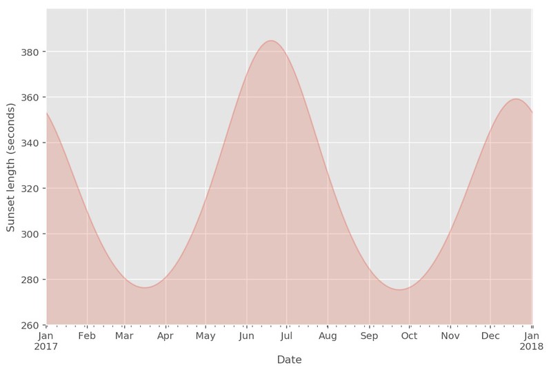
So from the graph above, it can be seen that there are two minima in the year where the sun sets the fastest - the middle of March and towards the end of September. The third week in June gives us the longest sunset, with the third week of December the second but smaller maximum of the year. These all correspond with the equinoxes and solstices as you would expect.
Conclusion
So there it is, fun times spent with PyEphem and our local star, and I’ve learned a thing or two along the way. I’ve got a few ideas for another article on this subject at some point, so keep your eyes peeled!
Comments
comments powered by Disqus